Tip

Run this Jupyter Notebook locally: Download Notebook

Tutorial kpm_tools.bloch

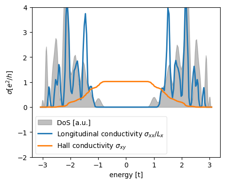
When computing the Kubo-Bastin conductivity with kwant.kpm.conductivity, the boundary effects are important. Actually, for any open boundary system, the (overall) Hall conductivity will be zero within all gaps, topological and trivial ones.

A workaround is to compute the conductivity at the bulk of the sample, to avoid boundary effects. This implies extra care on defining the KPM vectors, and the need for a larger system such that boundaries are far enough from the ‘bulk’ where the conductivity is computed.

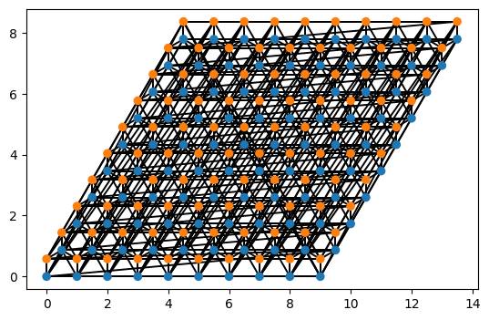
To address these issues, we can define a system with periodic boundary conditions, in which case we also need periodic velocity operators. The exact shape of the periodic operators depends on the details of the system and on the edges that are wrapped around with kwant.wraparound. The module kpm_tools.bloch takes care of correctly defining periodic velocity operators for any wrapped around system.

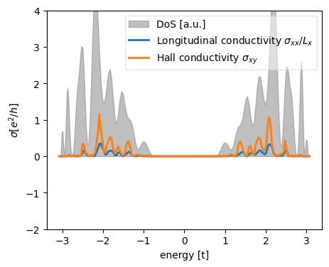
Here we will demonstrate the bloch module using a system with periodic boundary conditions to get the periodic velocity operators. If we would use the non-periodic velocity operators the results would be inconsistent.

This is evident when comparing the Kubo-Bastin longitudinal and Hall conductivity for a small topological system.

First some basic imports and plotting functions

import numpy as np
import kwant
from kpm_tools import bloch
from kpm_tools.bloch import wrap_velocity
from kpm_tools.hamiltonians import haldane_pbc

# plotting
import matplotlib.pyplot, matplotlib.backends
import matplotlib.pyplot as plt
import holoviews as hv
hv.notebook_extension()


def plot_dos_and_curves(dos, labels_to_data, ylabel="DoS [a.u.]"):
    plt.figure(figsize=(5,4))
    plt.fill_between(dos[0], dos[1], label="DoS [a.u.]",
                     alpha=0.5, color='gray')
    for label, (x, y) in labels_to_data:
        plt.plot(x, y, label=label, linewidth=2)
    plt.legend(framealpha=0.5)
    plt.xlabel("energy [t]")
    plt.ylabel(ylabel)

    plt.ylim(-2, 4)

Define a periodic Haldane topological system

lx = 10
ly = 10
trans_symm = [(lx, 0), (0, ly)]
lat, syst = haldane_pbc(trans_symm, return_builder=True)


fsyst = kwant.wraparound.wraparound(syst).finalized()

norbs = fsyst.sites[0].family.norbs
bounds = (-3.1, 3.1)


params = dict(zip(fsyst._momentum_names, (0, 0)))


kwant.plot(fsyst);

Define periodic velocity operators on the periodic system

velocity_builder = wrap_velocity(syst)
vx = velocity_builder.hamiltonian_submatrix(params=dict(k_x=0, k_y=0, direction=[1, 0]), sparse=True)
vy = velocity_builder.hamiltonian_submatrix(params=dict(k_x=0, k_y=0, direction=[0, 1]), sparse=True)

Use periodic velocity operators

(in a periodic system)

s_factory = kwant.kpm.LocalVectors(fsyst, where=None)
vectors = list(s_factory)
num_vectors = len(vectors)

# number of sites per vector
norm_v = np.linalg.norm(vectors[0]) ** 2

cond_xx = kwant.kpm.conductivity(
    fsyst, params=params,
    bounds=bounds,
    alpha=vx,
    beta=vx,
    mean=False,
    num_vectors=num_vectors,
    vector_factory=vectors)

cond_xy = kwant.kpm.conductivity(
    fsyst, params=params,
    alpha=vx,
    beta=vy,
    mean=False,
    num_vectors=num_vectors,
    vector_factory=vectors
)

energies = cond_xx.energies
cond_array_xx = np.array([cond_xx(e, temperature=0.0) for e in energies]).real
cond_array_xy = np.array([cond_xy(e, temperature=0.0) for e in energies]).real

# area of the unit cell per site
area_per_site = np.abs(np.cross(*lat.prim_vecs)) / len(lat.sublattices)
cond_array_xx /= area_per_site
cond_array_xy /= area_per_site

cond_array_xx = cond_array_xx / norm_v
cond_array_xy = cond_array_xy / norm_v

spectrum = kwant.kpm.SpectralDensity(fsyst, params=params)

plot_dos_and_curves(
    (spectrum.energies, spectrum.densities.real / (lx * ly / 3)),
    [
        (r'Longitudinal conductivity $\sigma_{xx}/L_x$',
         (spectrum.energies, cond_array_xx.mean(1) / (lx))),
        (r'Hall conductivity $\sigma_{xy}$',
         (spectrum.energies, cond_array_xy.mean(1)))],
    ylabel=r'$\sigma [e^2/h]$'
);

Use open boundary velocity operators

(in a periodic system..! don’t expect correct results)

s_factory = kwant.kpm.LocalVectors(fsyst, where=None)
vectors = list(s_factory)
num_vectors = len(vectors)

# number of sites per vector
norm_v = np.linalg.norm(vectors[0]) ** 2

cond_xx = kwant.kpm.conductivity(
    fsyst, params=params,
    bounds=bounds,
    alpha='x',
    beta='x',
    mean=False,
    num_vectors=num_vectors,
    vector_factory=vectors)

cond_xy = kwant.kpm.conductivity(
    fsyst, params=params,
    alpha='x',
    beta='y',
    mean=False,
    num_vectors=num_vectors,
    vector_factory=vectors
)

energies = cond_xx.energies
cond_array_xx = np.array([cond_xx(e, temperature=0.0) for e in energies]).real
cond_array_xy = np.array([cond_xy(e, temperature=0.0) for e in energies]).real

# area of the unit cell per site
area_per_site = np.abs(np.cross(*lat.prim_vecs)) / len(lat.sublattices)
cond_array_xx /= area_per_site
cond_array_xy /= area_per_site

cond_array_xx = cond_array_xx / norm_v
cond_array_xy = cond_array_xy / norm_v

spectrum = kwant.kpm.SpectralDensity(fsyst, params=params)

plot_dos_and_curves(
    (spectrum.energies, spectrum.densities.real / (lx * ly / 3)),
    [
        (r'Longitudinal conductivity $\sigma_{xx} / L_x$',
         (spectrum.energies, cond_array_xx.mean(1) / (lx))),
        (r'Hall conductivity $\sigma_{xy}$',
         (spectrum.energies, cond_array_xy.mean(1)))],
    ylabel=r'$\sigma [e^2/h]$'
);